About Intrinsic Dimension

Modern parameter-efficient fine-tuning (PEFT) techniques are built on a powerful foundational discovery: massive neural networks possess a remarkably low intrinsic dimension. In this article, we break down exactly what intrinsic dimension means and explore the empirical proofs that make efficient fine-tuning possible.

Background: Model Size Scaling

With the rapid growth of computational resources, there are in general three directions to scale model performance:

1. Data
2. Model size
3. Compute

The relative importance of each dimension remains an open question. Nevertheless, we have witnessed a rapid growth in model size over recent years.

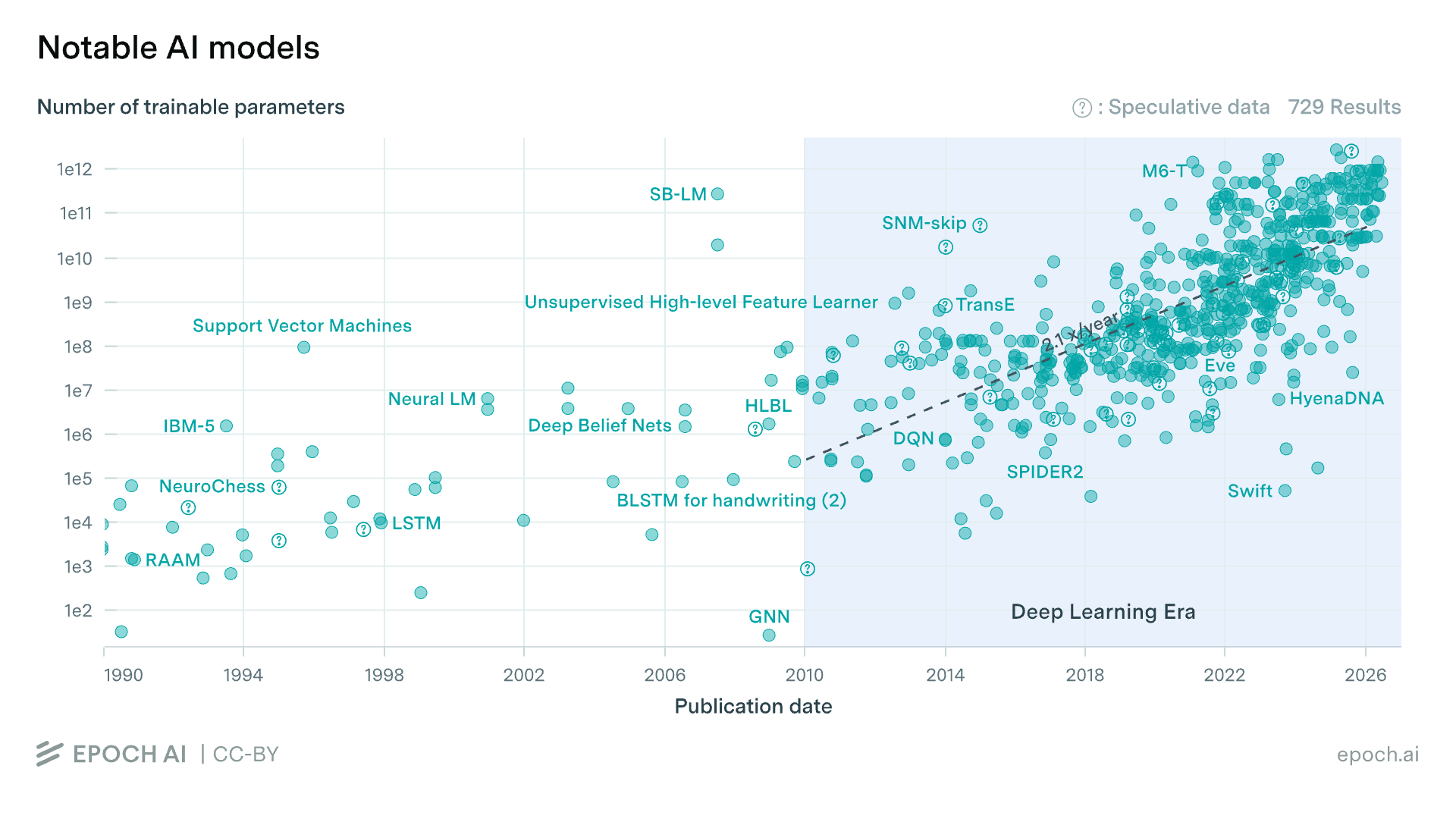
Models with billions to trillions of parameters have become the status quo. This begs the question: how many parameters are actually required?

Intrinsic Dimension

In mathematics, the intrinsic dimension of a subset is the minimal number of variables needed to represent the subset. It can be used as a measure of the complexity of the data set or signal.

In the context of machine learning, the intrinsic dimension of a model is defined as the minimum number of parameters required to achieve a solution [5]. Let’s look at a toy example.

A Toy Example

Consider a simple linear task where we seek a parameter vector $\Theta \in \mathbb{R}^3$:

We define the objective function as the squared error:

Minimizing this loss implies we want to find a $\Theta$ whose elements sum up to 1.

The Naive Approach

A straightforward approach is to optimize in the ambient space. We initialize at a random point $\Theta_{(0)} \sim \mathcal{N}(\mathbf{0},\mathbf{I}_3)$ and perform gradient descent in $\mathbb{R}^3$.

This solution is simple enough. The ambient dimension is 3, and the search space is $\mathbb{R}^3$. Is there an alternative approach with smaller search space?

Solution in 1D Subspace

Now let’s look at the objective landscape. The solution set is a 2D affine plane defined by $\theta_1 + \theta_2 + \theta_3 = 1$. In $\mathbb{R}^3$, any random 1D subspace (a line passing through the origin) will almost surely (probability = 1) intersect this 2D plane.

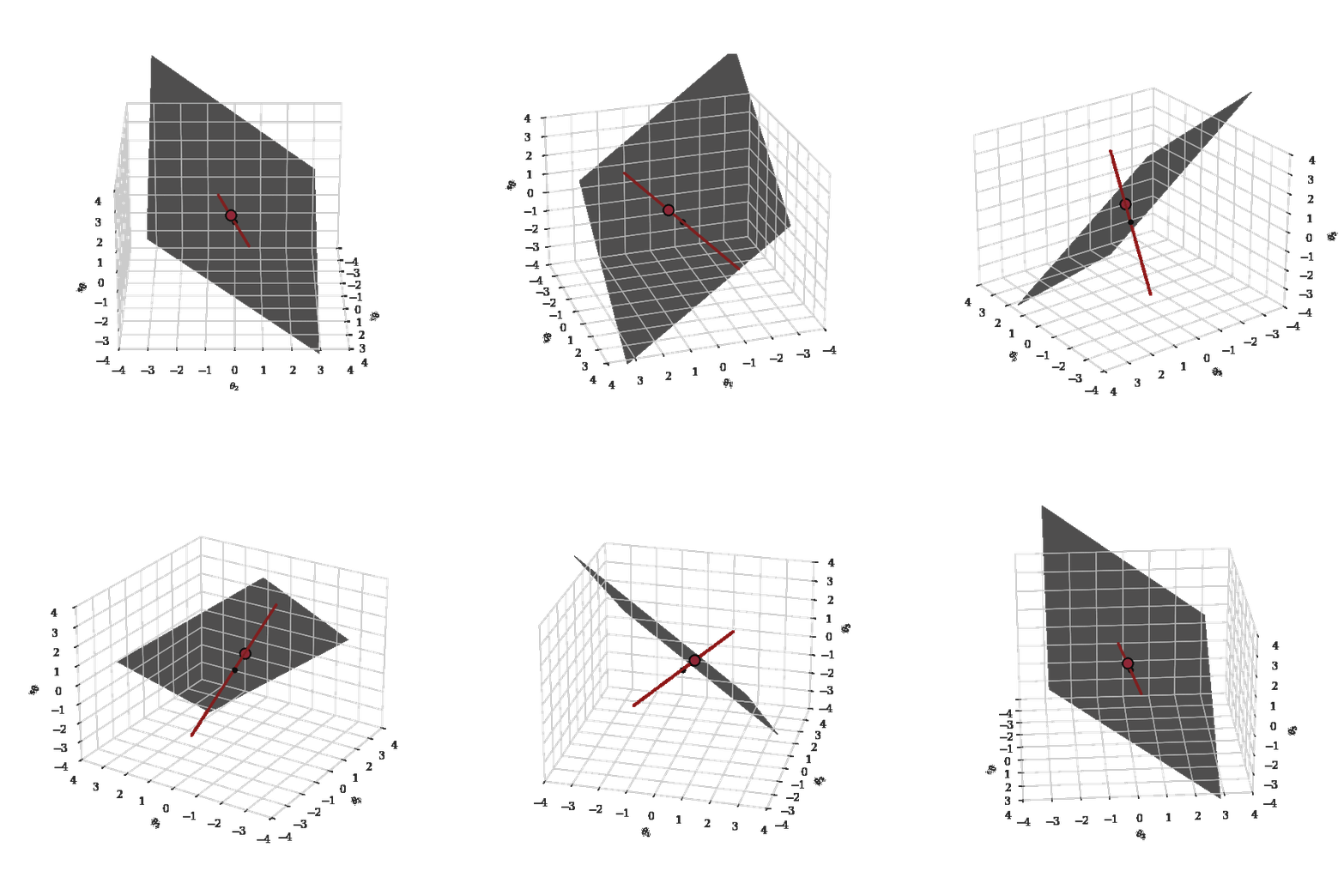
Therefore, we can constrain our search to a random 1D direction. Let $\mathbf{P} \sim \mathcal{N}(\mathbf{0},\mathbf{I}_3) \in \mathbb{R}^3$ be a fixed random vector. We now search for a single scalar multiplier $\lambda \in \mathbb{R}$ such that:

We have reduced the optimization problem from searching in $\mathbb{R}^3$ to searching along the line defined by $\mathbf{P}$ (i.e., search space becomes $\mathbb{R}$).

An optimal solution $\Theta^*$ exists for any random vector $\mathbf{P}$, provided $p_1 + p_2 + p_3 \neq 0$, which occurs with probability 1 for a random Gaussian initialization.

Since we can reach a global optimum $\mathcal{L}(\Theta) = 0$ by searching only one degree of freedom, the intrinsic dimension of this problem is 1.

Beyond Low-Dimensional Objective Landscape

Through this simple toy problem, we see that a 3D objective landscape can be solved with just a 1D search. But how does this extend to a deep neural network with billions of parameters?

The beauty of this concept, as we will see, is that the core mathematics do not change, they simply operate on a larger scale.

In our toy problem, the solution was a flat 2D plane. Because it stretched infinitely, our random 1D line was guaranteed to hit it. The loss landscapes of over-parameterized neural networks behave similarly [3]. They are not filled with isolated global minima. Instead, the solutions form vast, interconnected, flat manifolds. If this solution valley is vast enough, and a random multi-dimensional slice of the network has enough dimensions, that slice is virtually guaranteed to intersect the solution valley.

However, measuring the intrinsic dimension of a high-dimensional landscape is not easy. We can no longer visualize the space to derive the solution analytically. To bridge this gap, Uber AI Labs presented an elegant method in their 2018 ICLR paper to systematically measure the intrinsic dimension of these massive objective landscapes.

Measuring the Intrinsic Dimension of Objective Landscape

Li et al. from Uber AI Labs [5] proposed a method to measure the intrinsic dimension of a high-dimensional objective landscape.

In our toy problem, we searched for a scalar $\lambda$ to multiply by a random 1D vector $\mathbf{P}$. To scale this up to a massive neural network, we upgrade the scalar $\lambda$ to a small vector, and our random vector $\mathbf{P}$ to a random matrix.

Let $D$ be the total number of parameters in a neural network (the ambient dimension, e.g., 1M). Let $d \ll D$ be a much smaller number (the subspace dimension we want to test, e.g., 1K).

Instead of searching the full $D$-dimensional space, we define our network parameters $\Theta^{(D)}$ as:

Let’s break down this equation:

• $\Theta_0^{(D)}$ is the random initialization of the network (the starting point).
• $\mathbf{P}$ is a randomly initialized $D \times d$ projection matrix. This defines our random $d$-dimensional subspace (just like our random 1D line $\mathbf{P}$ in the toy example).
• $\theta^{(d)}$ is the small $d$-dimensional vector we are going to optimize (just like our scalar $\lambda$). It is initialized to all zeros, meaning training begins exactly at $\Theta_0^{(D)}$.

During training, we completely freeze the starting weights $\Theta_0^{(D)}$ and the random projection matrix $\mathbf{P}$. The only thing the optimizer is allowed to update is the small vector $\theta^{(d)}$.

To find the intrinsic dimension, we start with a small $d$, train the model by optimizing only $\theta^{(d)}$, and compare it against the baseline performance of a fully trained network. We gradually increase $d$ until we reach a point where the subspace-trained model is able to achieve a satisfactory solution (e.g., 90% of the baseline performance).

The minimum $d$ at which the model consistently solves the problem is defined as the intrinsic dimension of the objective landscape.

Intrinsic Dimensionality of Model Fine-tuning

Facebook AI [1] used a very similar method to measure the intrinsic dimension of language model fine-tuning. While the core concept remains the exact same as the Uber AI method, there are two primary differences required to scale this to massive transformer models:

• The Fastfood Transform [4]: Instead of using a standard random projection matrix ($\mathbf{P}$), they use the Fastfood transform to drastically reduce both the memory footprint and computational complexity of the projection.
• Structure-Aware Projection: Rather than applying a single, uniform global projection, they distribute the subspace parameters dynamically across the network. This accounts for the fact that different layers in attention-based pre-trained models have distinct “specializations”.

Ultimately, the underlying philosophy holds true: massive models can be effectively fine-tuned by optimizing only a tiny fraction of their parameters. For more details, I highly recommend reading their original paper.

Findings and Insights

Here are the most interesting takeaways presented in these papers:

• Intrinsic dimension is proportional to task difficulty [5].
• The intrinsic dimension isn’t just about the dataset. It is deeply tied to the architecture of the network [5]. Choosing the right inductive bias (e.g., using CNN for image tasks instead of fully-connected network) reduces the intrinsic dimension.
• RoBERTa-Large has 355 million parameters. On the MRPC binary classification task, the $d_{90}$ (the dimension needed to reach 90% performance) is around 200. That is $0.000056\%$ of the full parameter [1].
• Larger pre-trained models require lower intrinsic dimension to fine-tune for downstream tasks [1]. This might sound counterintuitive, but it reflects that large pre-trained models are incredible initializers, making them easier to adapt to downstream tasks.
• LLMs have a remarkably low intrinsic dimension [1]. This inspired the invention of LoRA, and is the fundamental reason we are able to efficiently fine-tune large models on standard consumer hardware.

Conclusion

This concept of low intrinsic dimension is the foundation of parameter-efficient fine-tuning (PEFT) techniques. Because large-scale pre-training compresses the search space, adapting a model requires updating only a tiny fraction of its parameters. Ultimately, this theoretical breakthrough gave rise to methods like LoRA, allowing us to efficiently fine-tune massive models on standard consumer hardware.

References

- Aghajanyan et al., “Intrinsic Dimensionality Explains the Effectiveness of Language Model Fine-Tuning”, IJCNLP 2021.
- Epoch AI, “Data on AI Models”, retrieved from https://epoch.ai/data/ai-models, 2026.
- Garipov et al., “Loss Surfaces, Mode Connectivity, and Fast Ensembling of DNNs”, NeurIPS 2018.
- Le et al., “Fastfood: approximating kernel expansions in loglinear time”, ICML 2013.
- Li et al., “Measuring the Intrinsic Dimension of Objective Landscapes”, ICLR 2018.